Calculation of confidence intervals

The lmfit confidence module allows you to explicitly calculate confidence intervals for variable parameters. For most models, it is not necessary: the estimation of the standard error from the estimated covariance matrix is normally quite good.

But for some models, e.g. a sum of two exponentials, the approximation begins to fail. For this case, lmfit has the function conf_interval() to calculate confidence intervals directly. This is substantially slower than using the errors estimated from the covariance matrix, but the results are more robust.

Method used for calculating confidence intervals

The F-test is used to compare our null model, which is the best fit we have found, with an alternate model, where one of the parameters is fixed to a specific value. The value is changed until the difference between \(\chi^2_0\) and \(\chi^2_{f}\) can’t be explained by the loss of a degree of freedom within a certain confidence.

\[F(P_{fix},N-P) = \left(\frac{\chi^2_f}{\chi^2_{0}}-1\right)\frac{N-P}{P_{fix}}\]

N is the number of data-points, P the number of parameter of the null model. \(P_{fix}\) is the number of fixed parameters (or to be more clear, the difference of number of parameters between our null model and the alternate model).

Adding a log-likelihood method is under consideration.

A basic example

First we create an example problem:

>>> import lmfit
>>> import numpy as np
>>> x = np.linspace(0.3,10,100)
>>> y = 1/(0.1*x)+2+0.1*np.random.randn(x.size)
>>> p = lmfit.Parameters()
>>> p.add_many(('a', 0.1), ('b', 1))
>>> def residual(p):
...    a = p['a'].value
...    b = p['b'].value
...    return 1/(a*x)+b-y

before we can generate the confidence intervals, we have to run a fit, so that the automated estimate of the standard errors can be used as a starting point:

>>> mi = lmfit.minimize(residual, p)
>>> lmfit.printfuncs.report_fit(mi.params)
[Variables]]
    a:   0.09943895 +/- 0.000193 (0.19%) (init= 0.1)
    b:   1.98476945 +/- 0.012226 (0.62%) (init= 1)
[[Correlations]] (unreported correlations are <  0.100)
    C(a, b)                      =  0.601

Now it is just a simple function call to calculate the confidence intervals:

>>> ci = lmfit.conf_interval(mi)
>>> lmfit.printfuncs.report_ci(ci)
     99.70%    95.00%    67.40%     0.00%    67.40%    95.00%    99.70%
a   0.09886   0.09905   0.09925   0.09944   0.09963   0.09982   0.10003
b   1.94751   1.96049   1.97274   1.97741   1.99680   2.00905   2.02203

This shows the best-fit values for the parameters in the 0.00% column, and parameter values that are at the varying confidence levels given by steps in \(\sigma\). As we can see, the estimated error is almost the same, and the uncertainties are well behaved: Going from 1 \(\sigma\) (68% confidence) to 3 \(\sigma\) (99.7% confidence) uncertainties is fairly linear. It can also be seen that the errors are fairy symmetric around the best fit value. For this problem, it is not necessary to calculate confidence intervals, and the estimates of the uncertainties from the covariance matrix are sufficient.

An advanced example

Now we look at a problem where calculating the error from approximated covariance can lead to misleading result – two decaying exponentials. In fact such a problem is particularly hard for the Levenberg-Marquardt method, so we fitst estimate the results using the slower but robust Nelder-Mead method, and then use Levenberg-Marquardt to estimate the uncertainties and correlations:

>>> x = np.linspace(1, 10, 250)
>>> np.random.seed(0)
>>> y = 3.0*np.exp(-x/2) -5.0*np.exp(-(x-0.1)/10.) + 0.1*np.random.randn(len(x))
>>>
>>> p = lmfit.Parameters()
>>> p.add_many(('a1', 4.), ('a2', 4.), ('t1', 3.), ('t2', 3.))
>>>
>>> def residual(p):
...    v = p.valuesdict()
...    return v['a1']*np.exp(-x/v['t1']) + v['a2']*np.exp(-(x-0.1)/v['t2'])-y
>>>
>>> # first solve with Nelder-Mead
>>> mi = lmfit.minimize(residual, p, method='Nelder')
>>> # then solve with Levenberg-Marquardt
>>> mi = lmfit.minimize(residual, p)
>>>
>>> lmfit.printfuncs.report_fit(mi.params, min_correl=0.5)

[[Variables]]
    a1:   2.98622120 +/- 0.148671 (4.98%) (init= 2.986237)
    a2:  -4.33526327 +/- 0.115275 (2.66%) (init=-4.335256)
    t1:   1.30994233 +/- 0.131211 (10.02%) (init= 1.309932)
    t2:   11.8240350 +/- 0.463164 (3.92%) (init= 11.82408)
[[Correlations]] (unreported correlations are <  0.500)
    C(a2, t2)                    =  0.987

Again we call conf_interval(), this time with tracing and only for 1- and 2 \(\sigma\):

>>> ci, trace = lmfit.conf_interval(mi, sigmas=[0.68,0.95], trace=True, verbose=False)
>>> lmfit.printfuncs.report_ci(ci)

      95.00%    68.00%     0.00%    68.00%    95.00%
a1   2.71850   2.84525   2.98622   3.14874   3.34076
a2  -4.63180  -4.46663  -4.35429  -4.22883  -4.14178
t2  10.82699  11.33865  11.78219  12.28195  12.71094
t1   1.08014   1.18566   1.38044   1.45566   1.62579

Comparing these two different estimates, we see that the estimate for a1 is reasonably well approximated from the covariance matrix, but the estimates for a2 and especially for t1, and t2 are very asymmetric and that going from 1 \(\sigma\) (68% confidence) to 2 \(\sigma\) (95% confidence) is not very predictable.

Now let’s plot a confidence region:

>>> import matplotlib.pylab as plt
>>> x, y, grid = lmfit.conf_interval2d(mi,'a1','t2',30,30)
>>> plt.contourf(x, y, grid, np.linspace(0,1,11))
>>> plt.xlabel('a1')
>>> plt.colorbar()
>>> plt.ylabel('t2')
>>> plt.show()

which shows the figure on the left below for a1 and t2, and for a2 and t2 on the right:

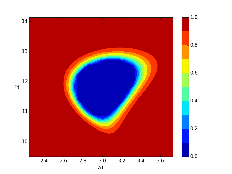
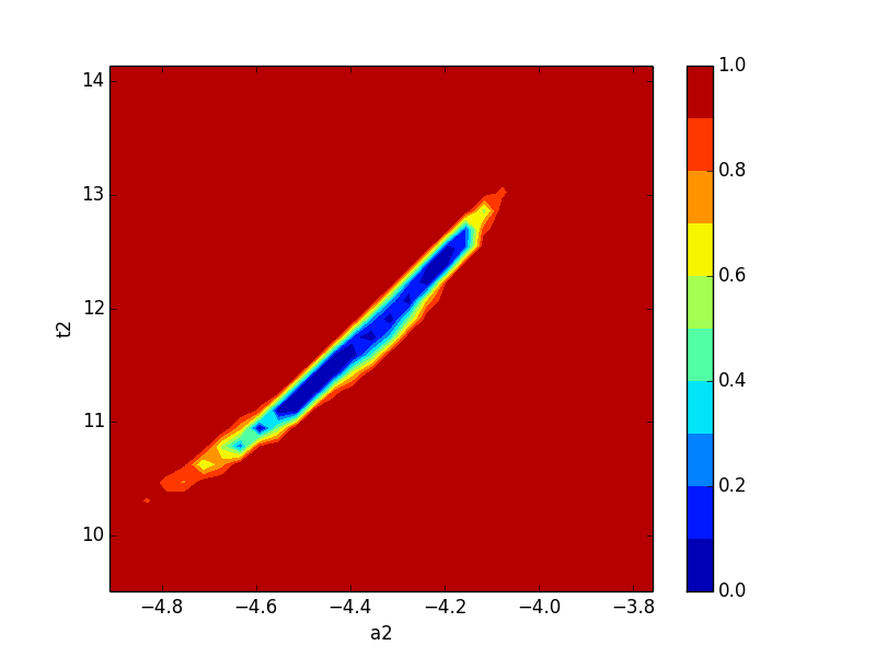
Neither of these plots is very much like an ellipse, which is implicitly assumed by the approach using the covariance matrix.

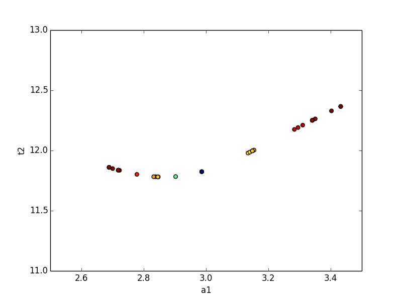
The trace returned as the optional second argument from conf_interval() contains a dictionary for each variable parameter. The values are dictionaries with arrays of values for each variable, and an array of corresponding probabilities for the corresponding cumulative variables. This can be used to show the dependence between two parameters:

>>> x, y, prob = trace['a1']['a1'], trace['a1']['t2'],trace['a1']['prob']
>>> x2, y2, prob2 = trace['t2']['t2'], trace['t2']['a1'],trace['t2']['prob']
>>> plt.scatter(x, y, c=prob ,s=30)
>>> plt.scatter(x2, y2, c=prob2, s=30)
>>> plt.gca().set_xlim((1, 5))
>>> plt.gca().set_ylim((5, 15))
>>> plt.xlabel('a1')
>>> plt.ylabel('t2')
>>> plt.show()

which shows the trace of values:

Documentation of methods

conf_interval(minimizer, p_names=None, sigmas=(0.674, 0.95, 0.997), trace=False, maxiter=200, verbose=False, prob_func=None)

Calculates the confidence interval for parameters from the given minimizer.

The parameter for which the ci is calculated will be varied, while the remaining parameters are re-optimized for minimizing chi-square. The resulting chi-square is used to calculate the probability with a given statistic e.g. F-statistic. This function uses a 1d-rootfinder from scipy to find the values resulting in the searched confidence region.

Parameters :

minimizer : Minimizer

The minimizer to use, should be already fitted via leastsq.

p_names : list, optional

Names of the parameters for which the ci is calculated. If None, the ci is calculated for every parameter.

sigmas : list, optional

The probabilities (1-alpha) to find. Default is 1,2 and 3-sigma.

trace : bool, optional

Defaults to False, if true, each result of a probability calculation is saved along with the parameter. This can be used to plot so called “profile traces”.

Returns :

output : dict

A dict, which contains a list of (sigma, vals)-tuples for each name.

trace_dict : dict

Only if trace is set true. Is a dict, the key is the parameter which was fixed.The values are again a dict with the names as keys, but with an additional key ‘prob’. Each contains an array of the corresponding values.

Other Parameters:  

maxiter : int

Maximum of iteration to find an upper limit.

prob_func : None or callable

Function to calculate the probability from the optimized chi-square. Default (None) uses built-in f_compare (F test).

verbose: bool :

print extra debuggin information. Default is False.

See also

conf_interval2d

Examples

>>> from lmfit.printfuncs import *
>>> mini = minimize(some_func, params)
>>> mini.leastsq()
True
>>> report_errors(params)
... #report
>>> ci = conf_interval(mini)
>>> report_ci(ci)
... #report

Now with quantiles for the sigmas and using the trace.

>>> ci, trace = conf_interval(mini, sigmas=(0.25, 0.5, 0.75, 0.999), trace=True)
>>> fixed = trace['para1']['para1']
>>> free = trace['para1']['not_para1']
>>> prob = trace['para1']['prob']

This makes it possible to plot the dependence between free and fixed.

conf_interval2d(minimizer, x_name, y_name, nx=10, ny=10, limits=None, prob_func=None)

Calculates confidence regions for two fixed parameters.

The method is explained in conf_interval: here we are fixing two parameters.

Parameters :

minimizer : minimizer

The minimizer to use, should be already fitted via leastsq.

x_name : string

The name of the parameter which will be the x direction.

y_name : string

The name of the parameter which will be the y direction.

nx, ny : ints, optional

Number of points.

limits : tuple: optional

Should have the form ((x_upper, x_lower),(y_upper, y_lower)). If not given, the default is 5 std-errs in each direction.

Returns :

x : (nx)-array

x-coordinates

y : (ny)-array

y-coordinates

grid : (nx,ny)-array

grid contains the calculated probabilities.

Other Parameters:  

prob_func : None or callable

Function to calculate the probability from the optimized chi-square. Default (None) uses built-in f_compare (F test).

Examples

>>> mini = minimize(some_func, params)
>>> mini.leastsq()
True
>>> x,y,gr = conf_interval2d('para1','para2')
>>> plt.contour(x,y,gr)