Modeling Data and Curve Fitting

A common use of least-squares minimization is curve fitting, where one has a parametrized model function meant to explain some phenomena and wants to adjust the numerical values for the model to most closely match some data. With scipy, such problems are commonly solved with scipy.optimize.curve_fit(), which is a wrapper around scipy.optimize.leastsq(). Since Lmfit’s minimize() is also a high-level wrapper around scipy.optimize.leastsq() it can be used for curve-fitting problems, but requires more effort than using scipy.optimize.curve_fit().

Here we discuss lmfit’s Model class. This takes a model function – a function that calculates a model for some data – and provides methods to create parameters for that model and to fit data using that model function. This is closer in spirit to scipy.optimize.curve_fit(), but with the advantages of using Parameters and lmfit.

In addition to allowing you turn any model function into a curve-fitting method, Lmfit also provides canonical definitions for many known line shapes such as Gaussian or Lorentzian peaks and Exponential decays that are widely used in many scientific domains. These are available in the models module that will be discussed in more detail in the next chapter (Built-in Fitting Models in the models module). We mention it here as you may want to consult that list before writing your own model. For now, we focus on turning python function into high-level fitting models with the Model class, and using these to fit data.

Example: Fit data to Gaussian profile

Let’s start with a simple and common example of fitting data to a Gaussian peak. As we will see, there is a buit-in GaussianModel class that provides a model function for a Gaussian profile, but here we’ll build our own. We start with a simple definition the model function:

>>> from numpy import sqrt, pi, exp, linspace
>>>
>>> def gaussian(x, amp, cen, wid):
...    return amp * exp(-(x-cen)**2 /wid)
...

that we want to use to fit to some data \(y(x)\) represented by the arrays y and x. Using scipy.optimize.curve_fit() makes this easy to do, allowing us to do something like:

>>> from scipy.optimize import curve_fit
>>>
>>> x, y = read_data_from_somewhere(....)
>>>
>>> init_vals = [5, 5, 1]     # for [amp, cen, wid]
>>> best_vals, covar = curve_fit(gaussian, x, y, p0=init_vals)
>>> print best_vals

That is, we read in data from somewhere, make an initial guess of the model values, and run scipy.optimize.curve_fit() with the model function, data arrays, and initial guesses. The results returned are the optimal values for the parameters and the covariance matrix. It’s simple and very useful. But it misses the benefits of lmfit.

To solve this with lmfit we would have to write an objective function. But such a function would be fairly simple (essentially, data - model, possibly with some weighting), and we would need to define and use appropriately named parameters. Though convenient, it is somewhat of a burden to keep the named parameter straight (on the other hand, with func:scipy.optimize.curve_fit you are required to remember the parameter order). After doing this a few times it appears as a recurring pattern, and we can imagine automating this process. That’s where the Model class comes in.

The Model allows us to easily wrap a model function such as the gaussian function. This automatically generate the appropriate residual function, and determines the corresponding parameter names from the function signature itself:

>>> from lmfit import Model
>>> gmod = Model(gaussian)
>>> gmod.param_names
set(['amp', 'wid', 'cen'])
>>> gmod.independent_vars)
['x']

The Model gmod knows the names of the parameters and the independent variables. By default, the first argument of the function is taken as the independent variable, held in independent_vars, and the rest of the functions positional arguments (and, in certain cases, keyword arguments – see below) are used for Parameter names. Thus, for the gaussian function above, the parameters are named amp, cen, and wid, and x is the independent variable – all taken directly from the signature of the model function. As we will see below, you can specify what the independent variable is, and you can add or alter parameters too.

On creation of the model, parameters are not created. The model knows what the parameters should be named, but not anything about the scale and range of your data. You will normally have to make these parameters and assign initial values and other attributes. To help you do this, each model has a make_params() method that will generate parameters with the expected names:

>>> params = gmod.make_params()

This creates the Parameters but doesn’t necessarily give them initial values – again, the model has no idea what the scale should be. You can set initial values for parameters with keyword arguments to make_params(), as with:

>>> params = gmod.make_params(cen=5, amp=200, wid=1)

or assign them (and other parameter properties) after the Parameters has been created.

A Model has several methods associated with it. For example, one can use the eval() method to evaluate the model or the fit() method to fit data to this model with a Parameter object. Both of these methods can take explicit keyword arguments for the parameter values. For example, one could use eval() to calculate the predicted function:

>>> x = linspace(0, 10, 201)
>>> y = gmod.eval(x=x, amp=10, cen=6.2, wid=0.75)

Admittedly, this a slightly long-winded way to calculate a Gaussian function. But now that the model is set up, we can also use its fit() method to fit this model to data, as with:

result = gmod.fit(y, x=x, amp=5, cen=5, wid=1)

Putting everything together, the script to do such a fit (included in the examples folder with the source code) is:

#!/usr/bin/env python
#<examples/doc_model1.py>
from numpy import sqrt, pi, exp, linspace, loadtxt
from lmfit import  Model

import matplotlib.pyplot as plt

data = loadtxt('model1d_gauss.dat')
x = data[:, 0]
y = data[:, 1]

def gaussian(x, amp, cen, wid):
    "1-d gaussian: gaussian(x, amp, cen, wid)"
    return (amp/(sqrt(2*pi)*wid)) * exp(-(x-cen)**2 /(2*wid**2))

gmod = Model(gaussian)
result = gmod.fit(y, x=x, amp=5, cen=5, wid=1)

print(result.fit_report())

plt.plot(x, y,         'bo')
plt.plot(x, result.init_fit, 'k--')
plt.plot(x, result.best_fit, 'r-')
plt.show()
#<end examples/doc_model1.py>

which is pretty compact and to the point. The returned result will be a ModelFit object. As we will see below, this has many components, including a fit_report() method, which will show:

[[Model]]
    gaussian
[[Fit Statistics]]
    # function evals   = 33
    # data points      = 101
    # variables        = 3
    chi-square         = 3.409
    reduced chi-square = 0.035
[[Variables]]
    amp:   8.88021829 +/- 0.113594 (1.28%) (init= 5)
    cen:   5.65866102 +/- 0.010304 (0.18%) (init= 5)
    wid:   0.69765468 +/- 0.010304 (1.48%) (init= 1)
[[Correlations]] (unreported correlations are <  0.100)
    C(amp, wid)                  =  0.577

The result will also have init_fit for the fit with the initial parameter values and a best_fit for the fit with the best fit parameter values. These can be used to generate the following plot:

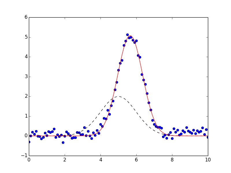
which shows the data in blue dots, the best fit as a solid red line, and the initial fit as a dashed black line.

We emphasize here that the fit to this model function was really performed with 2 lines of code:

gmod = Model(gaussian)
result = gmod.fit(y, x=x, amp=5, cen=5, wid=1)

These lines clearly express that we want to turn the gaussian function into a fitting model, and then fit the \(y(x)\) data to this model, starting with values of 5 for amp, 5 for cen and 1 for wid, and compare well to scipy.optimize.curve_fit():

best_vals, covar = curve_fit(gaussian, x, y, p0=[5, 5, 1])

except that all the other features of lmfit are included such as that the Parameters can have bounds and constraints and the result is a richer object that can be reused to explore the fit in more detail.

The Model class

The Model class provides a general way to wrap a pre-defined function as a fitting model.

class Model(func[, independent_vars=None[, param_names=None[, missing=None[, prefix=''[, name=None[, **kws]]]]]])

Create a model based on the user-supplied function. This uses introspection to automatically converting argument names of the function to Parameter names.

Parameters:

• func (callable) – model function to be wrapped
• independent_vars (None (default) or list of strings.) – list of argument names to func that are independent variables.
• param_names (None (default) or list of strings) – list of argument names to func that should be made into Parameters.
• missing (one of None (default), ‘none’, ‘drop’, or ‘raise’.) – how to handle missing values.
• prefix (string) – prefix to add to all parameter names to distinguish components in a CompositeModel.
• name (None or string.) – name for the model. When None (default) the name is the same as the model function (func).
• kws – additional keyword arguments to pass to model function.

Of course, the model function will have to return an array that will be the same size as the data being modeled. Generally this is handled by also specifying one or more independent variables.

Model class Methods

Model.eval(params=None[, **kws])

evaluate the model function for a set of parameters and inputs.

Parameters:

• params (None (default) or Parameters) – parameters to use for fit.
• kws – additional keyword arguments to pass to model function.

Returns:

ndarray for model given the parameters and other arguments.

If params is None, the values for all parameters are expected to be provided as keyword arguments. If params is given, and a keyword argument for a parameter value is also given, the keyword argument will be used.

Note that all non-parameter arguments for the model function – including all the independent variables! – will need to be passed in using keyword arguments.

Model.fit(data[, params=None[, weights=None[, method='leastsq'[, scale_covar=True[, iter_cb=None[, **kws]]]]]])

perform a fit of the model to the data array with a set of parameters.

Parameters:

• data (ndarray-like) – array of data to be fitted.
• params (None (default) or Parameters) – parameters to use for fit.
• weights (None (default) or ndarray-like.) – weights to use fit.
• method (string (default leastsq)) – name of fitting method to use. See Choosing Different Fitting Methods for details
• scale_covar (bool (default True)) – whether to automatically scale covariance matrix (leastsq only)
• iter_cb (callable or None) – function to be called at each fit iteration
• verbose (bool (default True)) – print a message when a new parameter is created due to a hint
• kws – additional keyword arguments to pass to model function.

Returns:

ModeFitResult object.

If params is None, the internal params will be used. If it is supplied, these will replace the internal ones. If supplied, weights must is an ndarray-like object of same size and shape as data.

Note that other arguments for the model function (including all the independent variables!) will need to be passed in using keyword arguments.

Model.guess(data, **kws)

Guess starting values for model parameters.

param data:data array used to guess parameter values type func:ndarray param kws:additional options to pass to model function. return:Parameters with guessed initial values for each parameter.

by default this is left to raise a NotImplementedError, but may be overwritten by subclasses. Generally, this method should take some values for data and use it to construct reasonable starting values for the parameters.

Model.make_params(**kws)

Create a set of parameters for model.

param kws:optional keyword/value pairs to set initial values for parameters. return:Parameters.

The parameters may or may not have decent initial values for each parameter.

Model.set_param_hint(name, value=None[, min=None[, max=None[, vary=True[, expr=None]]]])

set hints to use when creating parameters with Model.make_param() for the named parameter. This is especially convenient for setting initial values. The name can include the models prefix or not.

Parameters:

• name (string) – parameter name.
• value (float) – value for parameter
• min (None or float) – lower bound for parameter value
• max (None or float) – upper bound for parameter value
• vary (boolean) – whether to vary parameter in fit.
• expr (string) – mathematical expression for constraint

See Using parameter hints.

Model class Attributes

func

The model function used to calculate the model.

independent_vars

list of strings for names of the independent variables.

missing

describes what to do for missing values. The choices are

• None: Do not check for null or missing values (default)

• 'none': Do not check for null or missing values.

• 'drop': Drop null or missing observations in data. If pandas is

  installed, pandas.isnull is used, otherwise numpy.isnan is used.

• 'raise': Raise a (more helpful) exception when data contains null

  or missing values.

name

name of the model, used only in the string representation of the model. By default this will be taken from the model function.

opts

extra keyword arguments to pass to model function. Normally this will be determined internally and should not be changed.

param_hints

Dictionary of parameter hints. See Using parameter hints.

param_names

list of strings of parameter names.

prefix

prefix used for name-mangling of parameter names. The default is ‘’. If a particular Model has arguments amplitude, center, and sigma, these would become the parameter names. Using a prefix of g1_ would convert these parameter names to g1_amplitude, g1_center, and g1_sigma. This can be essential to avoid name collision in composite models.

Determining parameter names and independent variables for a function

The Model created from the supplied function func will create a Parameters object, and names are inferred from the function arguments, and a residual function is automatically constructed.

By default, the independent variable is take as the first argument to the function. You can explicitly set this, of course, and will need to if the independent variable is not first in the list, or if there are actually more than one independent variables.

If not specified, Parameters are constructed from all positional arguments and all keyword arguments that have a default value that is numerical, except the independent variable, of course. Importantly, the Parameters can be modified after creation. In fact, you’ll have to do this because none of the parameters have valid initial values. You can place bounds and constraints on Parameters, or fix their values.

Explicitly specifying independent_vars

As we saw for the Gaussian example above, creating a Model from a function is fairly easy. Let’s try another:

>>> def decay(t, tau, N):
...    return N*np.exp(-t/tau)
...
>>> decay_model = Model(decay)
>>> print decay_model.independent_vars
['t']
>>> for pname, par in decay_model.params.items():
...     print pname, par
...
tau <Parameter 'tau', None, bounds=[None:None]>
N <Parameter 'N', None, bounds=[None:None]>

Here, t is assumed to be the independent variable because it is the first argument to the function. The other function arguments are used to create parameters for the model.

If you want tau to be the independent variable in the above example, you can say so:

>>> decay_model = Model(decay, independent_vars=['tau'])
>>> print decay_model.independent_vars
['tau']
>>> for pname, par in decay_model.params.items():
...     print pname, par
...
t <Parameter 't', None, bounds=[None:None]>
N <Parameter 'N', None, bounds=[None:None]>

You can also supply multiple values for multi-dimensional functions with multiple independent variables. In fact, the meaning of independent variable here is simple, and based on how it treats arguments of the function you are modeling:

independent variable

a function argument that is not a parameter or otherwise part of the model, and that will be required to be explicitly provided as a keyword argument for each fit with Model.fit() or evaluation with Model.eval().

Note that independent variables are not required to be arrays, or even floating point numbers.

Functions with keyword arguments

If the model function had keyword parameters, these would be turned into Parameters if the supplied default value was a valid number (but not None, True, or False).

>>> def decay2(t, tau, N=10, check_positive=False):
...    if check_small:
...        arg = abs(t)/max(1.e-9, abs(tau))
...    else:
...        arg = t/tau
...    return N*np.exp(arg)
...
>>> mod = Model(decay2)
>>> for pname, par in mod.params.items():
...     print pname, par
...
t <Parameter 't', None, bounds=[None:None]>
N <Parameter 'N', 10, bounds=[None:None]>

Here, even though N is a keyword argument to the function, it is turned into a parameter, with the default numerical value as its initial value. By default, it is permitted to be varied in the fit – the 10 is taken as an initial value, not a fixed value. On the other hand, the check_positive keyword argument, was not converted to a parameter because it has a boolean default value. In some sense, check_positive becomes like an independent variable to the model. However, because it has a default value it is not required to be given for each model evaluation or fit, as independent variables are.

Defining a prefix for the Parameters

As we will see in the next chapter when combining models, it is sometimes necessary to decorate the parameter names in the model, but still have them be correctly used in the underlying model function. This would be necessary, for example, if two parameters in a composite model (see Composite Models : adding (or multiplying) Models or examples in the next chapter) would have the same name. To avoid this, we can add a prefix to the Model which will automatically do this mapping for us.

>>> def myfunc(x, amplitude=1, center=0, sigma=1):
...

>>> mod = Model(myfunc, prefix='f1_')
>>> for pname, par in mod.params.items():
...     print pname, par
...
f1_amplitude <Parameter 'f1_amplitude', None, bounds=[None:None]>
f1_center <Parameter 'f1_center', None, bounds=[None:None]>
f1_sigma <Parameter 'f1_sigma', None, bounds=[None:None]>

You would refer to these parameters as f1_amplitude and so forth, and the model will know to map these to the amplitude argument of myfunc.

Initializing model parameters

As mentioned above, the parameters created by Model.make_params() are generally created with invalid initial values of None. These values must be initialized in order for the model to be evaluated or used in a fit. There are four different ways to do this initialization that can be used in any combination:

1. You can supply initial values in the definition of the model function.
2. You can initialize the parameters when creating parameters with Model.make_params().
3. You can give parameter hints with Model.set_param_hint().
4. You can supply initial values for the parameters when you use the Model.eval() or Model.fit() methods.

Of course these methods can be mixed, allowing you to overwrite initial values at any point in the process of defining and using the model.

Initializing values in the function definition

To supply initial values for parameters in the definition of the model function, you can simply supply a default value:

>>> def myfunc(x, a=1, b=0):
>>>     ...

instead of using:

>>> def myfunc(x, a, b):
>>>     ...

This has the advantage of working at the function level – all parameters with keywords can be treated as options. It also means that some default initial value will always be available for the parameter.

Initializing values with Model.make_params()

When creating parameters with Model.make_params() you can specify initial values. To do this, use keyword arguments for the parameter names and initial values:

>>> mod = Model(myfunc)
>>> pars = mod.make_params(a=3, b=0.5)

Initializing values by setting parameter hints

After a model has been created, but prior to creating parameters with Model.make_params(), you can set parameter hints. These allows you to set not only a default initial value but also to set other parameter attributes controlling bounds, whether it is varied in the fit, or a constraint expression. To set a parameter hint, you can use Model.set_param_hint(), as with:

>>> mod = Model(myfunc)
>>> mod.set_param_hint('a', value = 1.0)
>>> mod.set_param_hint('b', value = 0.3, min=0, max=1.0)
>>> pars = mod.make_params()

Parameter hints are discussed in more detail in section Using parameter hints.

Initializing values when using a model

Finally, you can explicitly supply initial values when using a model. That is, as with Model.make_params(), you can include values as keyword arguments to either the Model.eval() or Model.fit() methods:

>>> y1 = mod.eval(x=x, a=7.0, b=-2.0)

>>> out = mod.fit(x=x, pars, a=3.0, b=-0.0)

These approaches to initialization provide many opportunities for setting initial values for parameters. The methods can be combined, so that you can set parameter hints but then change the initial value explicitly with Model.fit().

Using parameter hints

After a model has been created, you can give it hints for how to create parameters with Model.make_params(). This allows you to set not only a default initial value but also to set other parameter attributes controlling bounds, whether it is varied in the fit, or a constraint expression. To set a parameter hint, you can use Model.set_param_hint(), as with:

>>> mod = Model(myfunc)
>>> mod.set_param_hint('a', value = 1.0)
>>> mod.set_param_hint('b', value = 0.3, min=0, max=1.0)

Parameter hints are stored in a model’s param_hints attribute, which is simply a nested dictionary:

>>> print mod.param_hints
{'a': {'value': 1}, 'b': {'max': 1.0, 'value': 0.3, 'min': 0}}

You can change this dictionary directly, or with the Model.set_param_hint() method. Either way, these parameter hints are used by Model.make_params() when making parameters.

An important feature of parameter hints is that you can force the creation of new parameters with parameter hints. This can be useful to make derived parameters with constraint expressions. For example to get the full-width at half maximum of a Gaussian model, one could use a parameter hint of:

>>> mod = Model(gaussian)
>>> mod.set_param_hint('fwhm', expr='2.3548*sigma')

The ModelFit class

A ModelFit is the object returned by Model.fit(). It is a subclass of Minimizer, and so contains many of the fit results. Of course, it knows the Model and the set of Parameters used in the fit, and it has methods to evaluate the model, to fit the data (or re-fit the data with changes to the parameters, or fit with different or modified data) and to print out a report for that fit.

While a Model encapsulates your model function, it is fairly abstract and does not contain the parameters or data used in a particular fit. A ModelFit does contain parameters and data as well as methods to alter and re-do fits. Thus the Model is the idealized model while the ModelFit is the messier, more complex (but perhaps more useful) object that represents a fit with a set of parameters to data with a model.

A ModelFit object also includes basic methods for model selection: aic, bic and lik_ratio (see below).

A ModelFit has several attributes holding values for fit results, and several methods for working with fits.

class ModelFit

Model fit is intended to be created and returned by Model.fit().

ModelFit methods

These methods are all inherited from Minimize or from Model.

ModelFit.eval(**kwargs)

evaluate the model using the best-fit parameters and supplied independent variables. The **kwargs arguments can be used to update parameter values and/or independent variables.

ModelFit.eval_components(**kwargs)

evaluate each component of a CompositeModel, returning an ordered dictionary of with the values for each component model. The returned dictionary will have keys of the model prefix or (if no prefix is given), the model name. The **kwargs arguments can be used to update parameter values and/or independent variables.

ModelFit.fit(data=None[, params=None[, weights=None[, method=None[, **kwargs]]]])

fit (or re-fit), optionally changing data, params, weights, or method, or changing the independent variable(s) with the **kwargs argument. See Model.fit() for argument descriptions, and note that any value of None defaults to the last used value.

ModelFit.fit_report(modelpars=None[, show_correl=True[, `< min_correl=0.1]])

return a printable fit report for the fit with fit statistics, best-fit values with uncertainties and correlations. As with fit_report().

Parameters:

• modelpars – Parameters with “Known Values” (optional, default None)
• show_correl – whether to show list of sorted correlations [True]
• min_correl – smallest correlation absolute value to show [0.1]

ModelFit.aic()

Calculate the Akaike Information Criterion (AIC) of the model fit. AIC measures the relative quality of a statistical model for a given set of data. AIC balances between the fit of the model to the data and the complexity of the model; it can be used to prevent overfitting.

AIC is computed by AIC = n * log(rss/n) + 2k, where n is the number of data points, rss is the sum of residuals squares, and k in the number of estimated parameters.

AIC is used for model selection by selecting the model with the lowest AIC. It is a relative measure and as such can only be used to compare models. Compared to BIC, AIC can be considered less conservative, giving less weight to model simplicity (number of parameters) than BIC.

ModelFit.bic()

Calculate the Bayesian Information Criterion (BIC) of the model fit. BIC measures the relative quality of a statistical model for a given set of data. BIC balances between the fit of the model to the data and the complexity of the model; it can be used to prevent overfitting.

BIC is computed by BIC = n * log(rss/n) + log(n) k, where n is the number of data points, rss is the sum of residuals squares, and k in the number of estimated parameters.

BIC is used for model selection by selecting the model with the lowest BIC. BIC is a relative measure and as such can only be used to compare models. Compared to AIC, BIC can be considered more conservative, giving more weight to model simplicity (number of parameters) than AIC.

ModelFit.lik_ratio(other)

Calculate a likelihood ratio test for two model fits.

The likelihood ratio test is performed on two nested models (self is nested in other; that is, some of the parameters of other are fixed in self – the estimated paramters of self are a subset of the estimated parameters of other).

The null hypothesis of the test is that the nested model is true. The method returns the p-value of the test - the likelihood of getting the model fits we got, given the null hypothesis and the data.

The test calculates the statistic D = -2 log(lik0/lik1). lik0 and lik1 are the likelihoods of the nested and the nesting models, which are calculated as the reciprocal of the residual sum of squares.

By Wilks’s theorem, D is asymptotically chi-square distributed with df degrees of freedom, where df is the difference in number of parameters between the models; this allows the approximation of the p-value.

ModelFit attributes

best_fit

ndarray result of model function, evaluated at provided independent variables and with best-fit parameters.

best_values

dictionary with parameter names as keys, and best-fit values as values.

chisqr

floating point best-fit chi-square statistic.

covar

ndarray (square) covariance matrix returned from fit.

data

ndarray of data to compare to model.

errorbars

boolean for whether error bars were estimated by fit.

ier

integer returned code from scipy.optimize.leastsq().

init_fit

ndarray result of model function, evaluated at provided independent variables and with initial parameters.

init_params

initial parameters.

init_values

dictionary with parameter names as keys, and initial values as values.

iter_cb

optional callable function, to be called at each fit iteration. This must take take arguments of params, iter, resid, *args, **kws, where params will have the current parameter values, iter the iteration, resid the current residual array, and *args and **kws as passed to the objective function.

jacfcn

optional callable function, to be called to calculate jacobian array.

lmdif_message

string message returned from scipy.optimize.leastsq().

message

string message returned from minimize().

method

string naming fitting method for minimize().

model

instance of Model used for model.

ndata

integer number of data points.

nfev

integer number of function evaluations used for fit.

nfree

integer number of free parameters in fit.

nvarys

integer number of independent, freely varying variables in fit.

params

Parameters used in fit. Will have best-fit values.

redchi

floating point reduced chi-square statistic

residual

ndarray for residual.

scale_covar

boolean flag for whether to automatically scale covariance matrix.

success

boolean value of whether fit succeeded.

weights

ndarray (or None) of weighting values used in fit.

Composite Models : adding (or multiplying) Models

One of the more interesting features of the Model class is that Models can be added together or combined with basic algebraic operations (add, subtract, multiply, and divide) to give a composite model. The composite model will have parameters from each of the component models, with all parameters being available to influence the whole model. This ability to combine models will become even more useful in the next chapter, when pre-built subclasses of Model are discussed. For now, we’ll consider a simple example, and build a model of a Gaussian plus a line, as to model a peak with a background. For such a simple problem, we could just build a model that included both components:

def gaussian_plus_line(x, amp, cen, wid, slope, intercept):
    "line + 1-d gaussian"

    gauss = (amp/(sqrt(2*pi)*wid)) * exp(-(x-cen)**2 /(2*wid**2))
    line = slope * x + intercept
    return gauss + line

and use that with:

mod = Model(gaussian_plus_line)

But we already had a function for a gaussian function, and maybe we’ll discover that a linear background isn’t sufficient which would mean the model function would have to be changed. As an alternative we could define a linear function:

def line(x, slope, intercept):
    "a line"
    return slope * x + intercept

and build a composite model with just:

mod = Model(gaussian) + Model(line)

This model has parameters for both component models, and can be used as:

#!/usr/bin/env python
#<examples/model_doc2.py>
from numpy import sqrt, pi, exp, linspace, loadtxt
from lmfit import Model

import matplotlib.pyplot as plt

data = loadtxt('model1d_gauss.dat')
x = data[:, 0]
y = data[:, 1] + 0.25*x - 1.0

def gaussian(x, amp, cen, wid):
    "1-d gaussian: gaussian(x, amp, cen, wid)"
    return (amp/(sqrt(2*pi)*wid)) * exp(-(x-cen)**2 /(2*wid**2))

def line(x, slope, intercept):
    "line"
    return slope * x + intercept

mod = Model(gaussian) + Model(line)
pars  = mod.make_params( amp=5, cen=5, wid=1, slope=0, intercept=1)

result = mod.fit(y, pars, x=x)

print(result.fit_report())

plt.plot(x, y,         'bo')
plt.plot(x, result.init_fit, 'k--')
plt.plot(x, result.best_fit, 'r-')
plt.show()
#<end examples/model_doc2.py>

which prints out the results:

[[Model]]
    (Model(gaussian) + Model(line))
[[Fit Statistics]]
    # function evals   = 44
    # data points      = 101
    # variables        = 5
    chi-square         = 2.579
    reduced chi-square = 0.027
[[Variables]]
    amp:         8.45931061 +/- 0.124145 (1.47%) (init= 5)
    cen:         5.65547872 +/- 0.009176 (0.16%) (init= 5)
    intercept:  -0.96860201 +/- 0.033522 (3.46%) (init= 1)
    slope:       0.26484403 +/- 0.005748 (2.17%) (init= 0)
    wid:         0.67545523 +/- 0.009916 (1.47%) (init= 1)
[[Correlations]] (unreported correlations are <  0.100)
    C(amp, wid)                  =  0.666
    C(cen, intercept)            =  0.129

and shows the plot on the left.

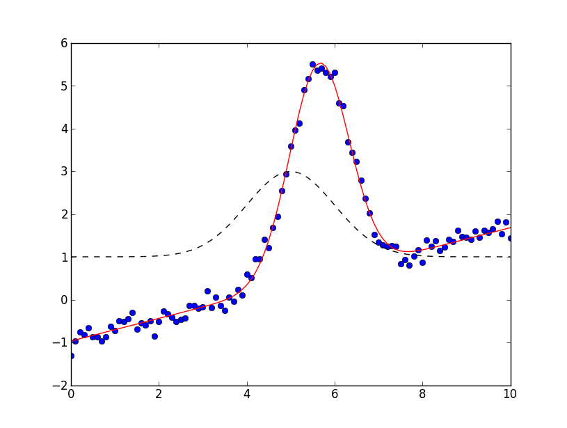
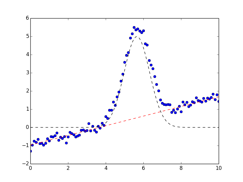
On the left, data is shown in blue dots, the total fit is shown in solid red line, and the initial fit is shown as a black dashed line. In the figure on the right, the data is again shown in blue dots, and the Gaussian component shown as a black dashed line, and the linear component shown as a red dashed line. These components were generated after the fit using the Models ModelFit.eval_components() method of the result:

comps = result.eval_components()

which returns a dictionary of the components, using keys of the model name (or prefix if that is set). This will use the parameter values in result.params and the independent variables (x) used during the fit. Note that while the ModelFit held in result does store the best parameters and the best estimate of the model in result.best_fit, the original model and parameters in pars are left unaltered.

You can apply this composite model to other data sets, or evaluate the model at other values of x. You may want to do this to give a finer or coarser spacing of data point, or to extrapolate the model outside the fitting range. This can be done with:

xwide = np.linspace(-5, 25, 3001)
predicted = mod.eval(x=xwide)

In this example, the argument names for the model functions do not overlap. If they had, the prefix argument to Model would have allowed us to identify which parameter went with which component model. As we will see in the next chapter, using composite models with the built-in models provides a simple way to build up complex models.

class CompositeModel(left, right, op[, **kws])

Create a composite model from two models (left and right and an binary operator (op). Additional keywords are passed to Model.

Parameters:

• left (Model) – left-hand side Model
• right (Model) – right-hand side Model
• op (callable, and taking 2 arguments (left and right).) – binary operator

Normally, one does not have to explicitly create a CompositeModel, as doing:

mod = Model(fcn1) + Model(fcn2) * Model(fcn3)

will automatically create a CompositeModel. In this example, mod.left will be Model(fcn1), mod.op will be operator.add(), and mod.right will be another CompositeModel that has a left attribute of Model(fcn2), an op of operator.mul(), and a right of Model(fcn3).

If you want to use a binary operator other than add, subtract, multiply, or divide that are supported through normal Python syntax, you’ll need to explicitly create a CompositeModel with the appropriate binary operator. For example, to convolve two models, you could define a simple convolution function, perhaps as:

import numpy as np
def convolve(dat, kernel):
    # simple convolution
    npts = min(len(dat), len(kernel))
    pad  = np.ones(npts)
    tmp  = np.concatenate((pad*dat[0], dat, pad*dat[-1]))
    out  = np.convolve(tmp, kernel, mode='valid')
    noff = int((len(out) - npts)/2)
    return (out[noff:])[:npts]

which extends the data in both directions so that the convolving kernel function gives a valid result over the data range. Because this function takes two array arguments and returns an array, it can be used as the binary operator. A full script using this technique is here:

#!/usr/bin/env python
#<examples/model_doc3.py>

import numpy as np
from lmfit import Model, CompositeModel
from lmfit.lineshapes import step, gaussian

import matplotlib.pyplot as plt

# create data from broadened step
npts = 201
x = np.linspace(0, 10, npts)
y = step(x, amplitude=12.5, center=4.5, sigma=0.88, form='erf')
y = y + np.random.normal(size=npts, scale=0.35)

def jump(x, mid):
    "heaviside step function"
    o = np.zeros(len(x))
    imid = max(np.where(x<=mid)[0])
    o[imid:] = 1.0
    return o

def convolve(arr, kernel):
    # simple convolution of two arrays
    npts = min(len(arr), len(kernel))
    pad  = np.ones(npts)
    tmp  = np.concatenate((pad*arr[0], arr, pad*arr[-1]))
    out  = np.convolve(tmp, kernel, mode='valid')
    noff = int((len(out) - npts)/2)
    return out[noff:noff+npts]
#
# create Composite Model using the custom convolution operator
mod  = CompositeModel(Model(jump), Model(gaussian), convolve)

pars = mod.make_params(amplitude=1, center=3.5, sigma=1.5, mid=5.0)

# 'mid' and 'center' should be completely correlated, and 'mid' is
# used as an integer index, so a very poor fit variable:
pars['mid'].vary = False

# fit this model to data array y
result =  mod.fit(y, params=pars, x=x)

print(result.fit_report())

plot_components = False

# plot results
plt.plot(x, y,         'bo')
if plot_components:
    # generate components
    comps = result.eval_components(x=x)
    plt.plot(x, 10*comps['jump'], 'k--')
    plt.plot(x, 10*comps['gaussian'], 'r-')
else:
    plt.plot(x, result.init_fit, 'k--')
    plt.plot(x, result.best_fit, 'r-')
plt.show()
# #<end examples/model_doc3.py>

which prints out the results:

[[Model]]
    (Model(jump) <function convolve at 0x109ee4488> Model(gaussian))
[[Fit Statistics]]
    # function evals   = 25
    # data points      = 201
    # variables        = 3
    chi-square         = 21.692
    reduced chi-square = 0.110
[[Variables]]
    amplitude:   0.62106099 +/- 0.001783 (0.29%) (init= 1)
    center:      4.49913218 +/- 0.009373 (0.21%) (init= 3.5)
    mid:         5 (fixed)
    sigma:       0.61936067 +/- 0.012977 (2.10%) (init= 1)
[[Correlations]] (unreported correlations are <  0.100)
    C(amplitude, center)         =  0.336
    C(amplitude, sigma)          =  0.274

and shows the plots:

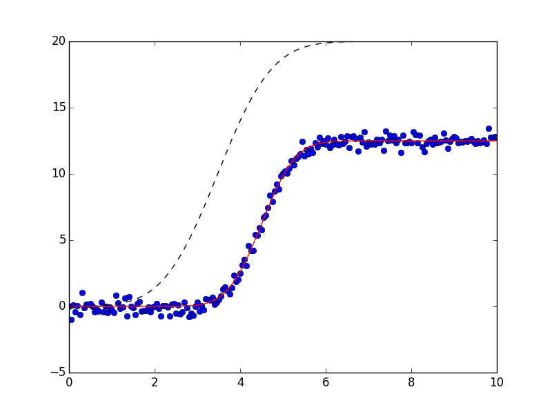
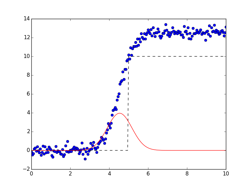
Using composite models with built-in or custom operators allows you to build complex models from testable sub-components.